Authors: Nils Thuerey
Here you can find an reference implementation of the ACM Transactions on Graphics paper Interpolations of Smoke and Liquid Simulations.
Download the sources here:
ofblend.tar.gz
(Note - this source code is based on mantaflow,
so it contains third party components; please check the respective source distribution webpages for details.)
You can just follow the mantaflow installation instructions.
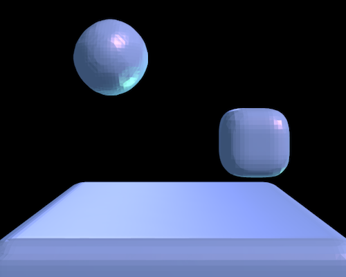
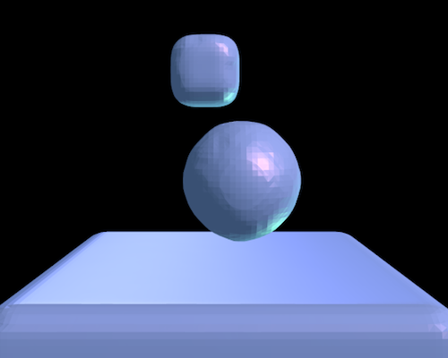
Run the two commands below to simulate two different liquid drop setups.
The first two images on the right illustrate the initial positions.
By default a relatively small
resolution of 40 cells is used, in order to keep the runtimes low. The following
commands assume that you built mantaflow in a separate directory next to source directory "mantaflowgit",
which also contains the scene files.
The two commands will generate a lower resolution 4D SDF ("out_r040_x000.uni" and "out_r040_x001.uni"
in this case), and a series of full resolution 3D SDFs ("outxl...").
./manta ../mantaflowgit/scenes/dataGen2Drop.py px 0 save4d 1 savehi 1
./manta ../mantaflowgit/scenes/dataGen2Drop.py px 1 save4d 1 savehi 1
The FlOF.py script includes all that is necessary to compute a space-time
deformation with optical flow. It also has hard coded settings to load the
data generated in the previous step. The two data points (0 and 1) will be
used as end-points for the calculations in the following.
./manta ../mantaflowgit/scenes/flof.py dataid0 0 dataid1 1 mode 1
This will take circa 2-3 minutes, and generate a 4D deformation field called "defo01_000_001_032_vel.uni".
the flof script has different modes: mode 1 calculates a deformation, mode 2 applies it for testing,
and mode 3 performs the full interpolation between multiple data points.
if you compiled the code with qt support, you can visually check the deformation with:
./manta ../mantaflowgit/scenes/flof.py dataid0 0 dataid1 1 mode 2 showgui 1
add an "alpha x" value (x between 0 and 100) to test intermediate deformations which are not appplied
with full strength.
The previous steps apply the deformation using the lower grid resolution (32 in this case).
You can test a one-way, high-resolution output with mode 3 using the following command:
./manta ../mantaflowgit/scenes/flof.py dataid0 0 dataid1 1 mode 3 showgui 1 alpha 50
To run the full pipeline as described in the paper, you also need a deformation
in the other direction. Run the following commands to generate and check it:
./manta ../mantaflowgit/scenes/flof.py dataid0 1 dataid1 0 mode 1
./manta ../mantaflowgit/scenes/flof.py dataid0 1 dataid1 0 mode 2 showgui 1
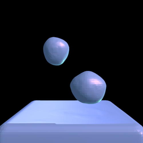
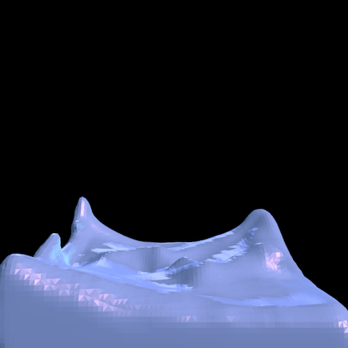
Now we have all components ready to generate a real output: the high-res input data,
and the deformations in both directions. The following command will apply
them with 50% strength, and save a sequence of png images. You can see a preview
on the right (the lower two images).
./manta ../mantaflowgit/scenes/flof.py flof.py mode 3 showgui 1 twoway 1 alpha 50 writepngs 1
To generate triangle meshes that could, e.g., be displayed and rendered in blender, add "trimesh 1".
This completes a full simple example.
Let me know how it works for you! If you have comments / questions, just send a mail to
"nils at thuerey dot de".
This work was funded by the ERC Starting Grant
realFlow.
|
 |
 |